Trying out new Tidymodels package: vetiver

Introduction

The Jan 11, 2022 Tidy Tuesday dataset provides an opportunity to try out the latest addition to the tidymodels ecosystem. The vetiver package is designed for easy model deployment & versioning.

First we’ll read in the dataset and explore it, create and compare some models, select a and deploy a final model as a versioned API using vetiver. The goal of this post isn’t to create the best model possible, though the modelling concepts and steps used here are also used when developing a “real” ML model. Instead the focus of this post is around deploying a model as an API using the vetiver package.

Explore the data

There are 2 datasets: colony and stressor; We will develop a model using stressors to predict colonies lost.

colony %>% get_table()

stressor %>% get_table()

colony %>%
  filter(state != 'United States') %>%
  group_by(year, state) %>%
  summarise(mean_loss = mean(colony_lost, na.rm = T),
            mean_pct_loss = mean(colony_lost_pct, na.rm = T)) %>% 
  hchart(., "heatmap", hcaes(x = year, y = state, value = mean_pct_loss)) %>%
  hc_title(text = "Percent of colony lost by state/year", align = "left")

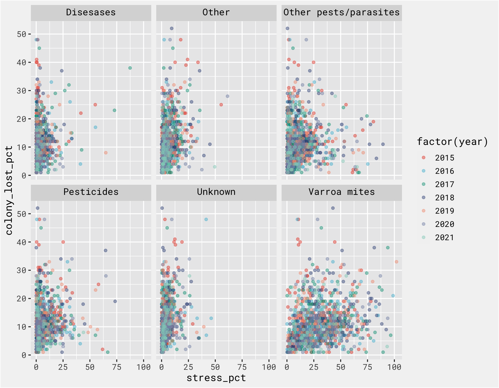
There is not a clear relationship between each stressor at the outcome, but the purpose of this isn’t to create a great model. We just need a model to get to the fun part of deploying it as an API and calling it to make predictions.

stressor %>%
  filter(state != 'United States') %>%
  inner_join(., colony) %>%
  ggplot(., aes(x = stress_pct, y = colony_lost_pct, color = factor(year))) + 
  geom_point(alpha = .45) + 
  # coord_equal() + 
  facet_wrap(vars(stressor)) +
  bg_theme(base_size = 13) + 
  ggsci::scale_color_npg()

Here we create the modeling dataset. We have some missing data so we can add a pre-processing step to address that.

model_data <- 
  colony %>%
  filter(state != 'United States') %>%
  select(year:state, colony_lost_pct) %>%
  inner_join(., stressor %>%
               pivot_wider(names_from = stressor, values_from = stress_pct)) %>%
  filter(!(is.na(colony_lost_pct))) %>%
  select(-c(year, state, months)) %>%
  select(colony_lost_pct, everything())

model_data %>% 
  get_table()

Develop models

Next step is to decide how we’re going to “spend” the data we have. We need to leave some data untouched when fitting and tuning the models in order to get a sense of how our final model will handle brand new data. The train data is used to tune the models and the test data is our holdout set, used only to evaluate the final model.

set.seed(1701)

splits <- 
  rsample::initial_split(model_data, strata = colony_lost_pct)

train <- 
  training(splits)

test <- 
  testing(splits)

splits

## <Training/Testing/Total>
## <856/287/1143>

We’ll need to tune some model hyperparameters, so we create some bootstrap resamples of the training data. We created 25 resamples, so each hyperparameter combination for each model will be fit and evaluated on each of the 25 splits.

folds <- 
  bootstraps(train, strata = colony_lost_pct, times = 25)

folds

## # Bootstrap sampling using stratification 
## # A tibble: 25 × 2
##    splits            id         
##    <list>            <chr>      
##  1 <split [856/307]> Bootstrap01
##  2 <split [856/310]> Bootstrap02
##  3 <split [856/330]> Bootstrap03
##  4 <split [856/322]> Bootstrap04
##  5 <split [856/310]> Bootstrap05
##  6 <split [856/314]> Bootstrap06
##  7 <split [856/310]> Bootstrap07
##  8 <split [856/316]> Bootstrap08
##  9 <split [856/312]> Bootstrap09
## 10 <split [856/309]> Bootstrap10
## # … with 15 more rows
## # ℹ Use `print(n = ...)` to see more rows

Here we so define some pre-processing steps using the recipes package`:

• median imputation for the missing observations
• center/scale all numeric predictors

recipe <- 
  recipe(colony_lost_pct ~ ., data = train) %>%
  step_impute_median(all_numeric_predictors()) %>%
  step_normalize(all_numeric_predictors()) 

recipe

## Recipe
## 
## Inputs:
## 
##       role #variables
##    outcome          1
##  predictor          6
## 
## Operations:
## 
## Median imputation for all_numeric_predictors()
## Centering and scaling for all_numeric_predictors()

Prep the recipe to make sure there are no issues with the pre-processing steps

prep(recipe) %>% 
  bake(new_data = NULL) %>% 
  get_table()

Three models are specified and combined with the recipe into a workflowset, which is a certain type of tidymodels object that makes tuning and comparing several models extremely easy.

lasso_rec <- 
  parsnip::linear_reg(mixture = 1, 
                      penalty = tune()) %>%
  set_engine("glmnet")

cubist_rec <- 
  cubist_rules(committees = tune(), 
               neighbors = tune()) %>% 
  set_engine("Cubist")

rf_rec <- 
  parsnip::rand_forest(mtry = tune(),
                       trees = 1000, 
                       min_n = tune()) %>%
  set_mode("regression") %>%
  set_engine("ranger")

workflows <- 
  workflow_set(
    preproc = list(recipe = recipe), 
    models = list(lasso = lasso_rec,
                  cubist = cubist_rec,
                  forest = rf_rec),
    cross = TRUE)

workflows

## # A workflow set/tibble: 3 × 4
##   wflow_id      info             option    result    
##   <chr>         <list>           <list>    <list>    
## 1 recipe_lasso  <tibble [1 × 4]> <opts[0]> <list [0]>
## 2 recipe_cubist <tibble [1 × 4]> <opts[0]> <list [0]>
## 3 recipe_forest <tibble [1 × 4]> <opts[0]> <list [0]>

Here we tune the models via grid search and check the results. We have a grid of size 10, which means each model is fit using 10 different hyperparameter combinations. That, combined with the 25 resamples per model, means we fit 250 models for each of the 3 models specified above for a total of 750 models.

cl <- 
  makeCluster(10)

doParallel::registerDoParallel(cl)

grid_ctrl <-
  control_grid(
    save_pred = TRUE,
    allow_par = TRUE,
    parallel_over = "everything",
    verbose = TRUE
  )

results <- 
  workflow_map(fn = "tune_grid",
               object = workflows,
               seed = 1837,
               verbose = T,
               control = grid_ctrl,
               grid = 10, 
               resamples = folds,
               metrics = metric_set(rmse, mae)
  )

stopCluster(cl)

workflowsets::rank_results(results, select_best = T, rank_metric = "rmse")

## # A tibble: 6 × 9
##   wflow_id      .config          .metric  mean std_err     n prepr…¹ model  rank
##   <chr>         <chr>            <chr>   <dbl>   <dbl> <int> <chr>   <chr> <int>
## 1 recipe_forest Preprocessor1_M… mae      4.79  0.0353    25 recipe  rand…     1
## 2 recipe_forest Preprocessor1_M… rmse     6.57  0.0716    25 recipe  rand…     1
## 3 recipe_lasso  Preprocessor1_M… mae      4.92  0.0390    25 recipe  line…     2
## 4 recipe_lasso  Preprocessor1_M… rmse     6.75  0.0780    25 recipe  line…     2
## 5 recipe_cubist Preprocessor1_M… mae      5.04  0.0545    25 recipe  cubi…     3
## 6 recipe_cubist Preprocessor1_M… rmse     6.94  0.0916    25 recipe  cubi…     3
## # … with abbreviated variable name ¹​preprocessor

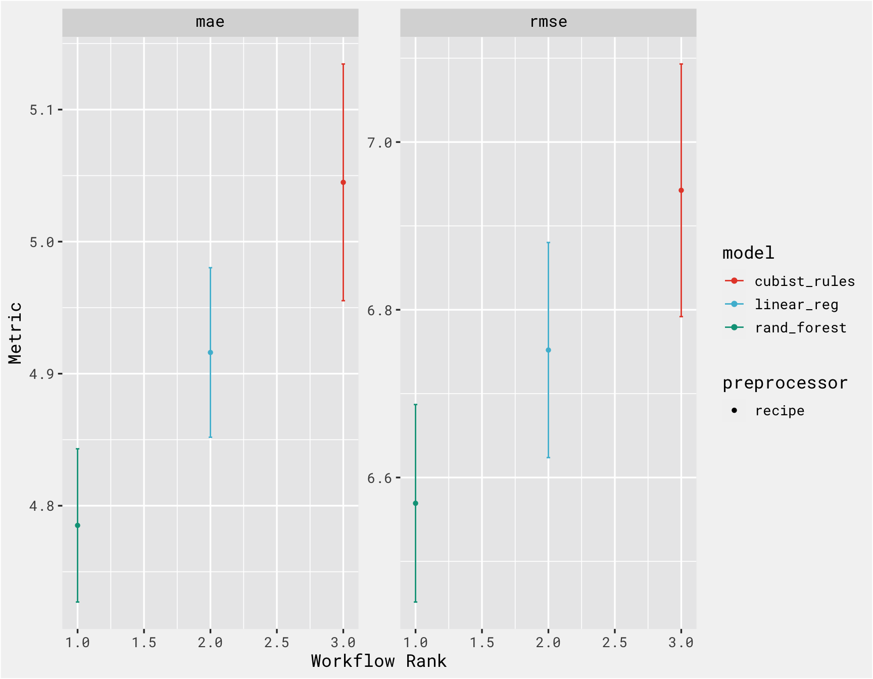
autoplot(results, select_best = T) +
  bg_theme(base_size = 13) + 
  ggsci::scale_color_npg()

Using vetiver

From the package website:

The goal of vetiver is to provide fluent tooling to version, share, deploy, and monitor a trained model. Functions handle both recording and checking the model’s input data prototype, and predicting from a remote API endpoint. The vetiver package is extensible, with generics that can support many kinds of models.

This is great because prepping a model for deployment and then managing the deployment/versioning can be a pain. vetiver takes a fitted workflow, so we choose the best model based on the plot above, and “finalize” it by “locking in” the hyperparameter values that of random forest model and fitting that model on training set (in reality though, you would typically tune and compare several models, select the best model, evaluate on the test set, finalize the model, deploy it, and then predict on new data as necessary. We don’t have any new data though, so we’re using the test dataset as our “new data”)

best_results <- 
  results %>% 
  extract_workflow_set_result("recipe_forest") %>% 
  select_best(metric = "rmse")

best_rf <- 
  parsnip::rand_forest(mtry = best_results$mtry,
                       trees = 1000, 
                       min_n = best_results$min_n) %>%
  set_mode("regression") %>%
  set_engine("ranger")

best_model <- 
  finalize_workflow(x = workflow() %>% add_recipe(recipe) %>% add_model(best_rf), 
                    parameters = best_results) %>%
  fit(train)

best_model

## ══ Workflow [trained] ══════════════════════════════════════════════════════════
## Preprocessor: Recipe
## Model: rand_forest()
## 
## ── Preprocessor ────────────────────────────────────────────────────────────────
## 2 Recipe Steps
## 
## • step_impute_median()
## • step_normalize()
## 
## ── Model ───────────────────────────────────────────────────────────────────────
## Ranger result
## 
## Call:
##  ranger::ranger(x = maybe_data_frame(x), y = y, mtry = min_cols(~best_results$mtry,      x), num.trees = ~1000, min.node.size = min_rows(~best_results$min_n,      x), num.threads = 1, verbose = FALSE, seed = sample.int(10^5,      1)) 
## 
## Type:                             Regression 
## Number of trees:                  1000 
## Sample size:                      856 
## Number of independent variables:  6 
## Mtry:                             1 
## Target node size:                 34 
## Variable importance mode:         none 
## Splitrule:                        variance 
## OOB prediction error (MSE):       43.64448 
## R squared (OOB):                  0.201183

Next we create vetiver object and pin to temp board. The piece of code at the end of this chunk creates a file for us called plumber.R and puts it in the working directory. This file contains the packages and files necessary to deploy the model as an API. But, first we can test it locally in the next step.

v <- 
  vetiver_model(model = best_model, 
                model_name = "lost-colony-model")

tmp <- 
  tempfile()

model_board <- 
  board_temp(versioned = TRUE)

model_board %>% 
  vetiver_pin_write(v)

model_board

#this creates a plumber file with a 'predict' endpoint
vetiver_write_plumber(board = model_board, 
                      name = "lost-colony-model",
                      file = here::here("2022", "plumber.R"))

Following the steps outlined here, we can run the API locally and call the /predict endpoint to apply our model on new data. First create the file called entrypoint.R and follow the instructions to run it as a local job. Paste the URL in vetiver_endpoint() below and retrieve your predictions using the test data!

endpoint <- 
  vetiver_endpoint("http://127.0.0.1:8251/predict")

endpoint

preds <- 
  predict(endpoint, test) %>%
  cbind(., test)

Ideally the points in the scatterplot would fall along, or near, the 45-degree line, so the model performance isn’t great. But we were able to successfully deploy it as an API and retrieve predictions!

preds %>%
  ggplot(., aes(x = colony_lost_pct, y = .pred)) + 
  geom_abline(col = bg_red, lty = 2) + 
  geom_point(alpha = 0.5, color = bg_green) + 
  coord_obs_pred() + 
  labs(x = "observed", y = "predicted", title = "predicted colony lost pct vs actual") + 
  bg_theme()