Comparing Traditional and Text-Based Models to Predict Chocolate Rating
By Brendan Graham in tidy tuesday tidymodels data science
January 18, 2022
The goal for this weeks analysis to compare 2 types of models for predicting chocolate ratings. I have read bout text based models but haven’t every attempted one, so in this analysis I will compare some text-based models with more traditional ML models.
The data is composed of 2,530 observations of 10 variables. There is some missing ingredients data, but all other columns are complete.
chocolate
## # A tibble: 2,530 × 10
##      ref company_manufacturer company_location review_date country_of_bean_orig…
##    <dbl> <chr>                <chr>                  <dbl> <chr>
##  1  2454 5150                 U.S.A.                  2019 Tanzania
##  2  2458 5150                 U.S.A.                  2019 Dominican Republic
##  3  2454 5150                 U.S.A.                  2019 Madagascar
##  4  2542 5150                 U.S.A.                  2021 Fiji
##  5  2546 5150                 U.S.A.                  2021 Venezuela
##  6  2546 5150                 U.S.A.                  2021 Uganda
##  7  2542 5150                 U.S.A.                  2021 India
##  8   797 A. Morin             France                  2012 Bolivia
##  9   797 A. Morin             France                  2012 Peru
## 10  1011 A. Morin             France                  2013 Panama
## # … with 2,520 more rows, and 5 more variables:
## #   specific_bean_origin_or_bar_name <chr>, cocoa_percent <chr>,
## #   ingredients <chr>, most_memorable_characteristics <chr>, rating <dbl>
skimr::skim_to_list(chocolate)
Variable type: character
| skim_variable | n_missing | complete_rate | min | max | empty | n_unique | whitespace |
|---|---|---|---|---|---|---|---|
| company_manufacturer | 0 | 1.00 | 2 | 39 | 0 | 580 | 0 |
| company_location | 0 | 1.00 | 4 | 21 | 0 | 67 | 0 |
| country_of_bean_origin | 0 | 1.00 | 4 | 21 | 0 | 62 | 0 |
| specific_bean_origin_or_bar_name | 0 | 1.00 | 3 | 51 | 0 | 1605 | 0 |
| cocoa_percent | 0 | 1.00 | 3 | 6 | 0 | 46 | 0 |
| ingredients | 87 | 0.97 | 4 | 14 | 0 | 21 | 0 |
| most_memorable_characteristics | 0 | 1.00 | 3 | 37 | 0 | 2487 | 0 |
Variable type: numeric
| skim_variable | n_missing | complete_rate | mean | sd | p0 | p25 | p50 | p75 | p100 | hist |
|---|---|---|---|---|---|---|---|---|---|---|
| ref | 0 | 1 | 1429.80 | 757.65 | 5 | 802 | 1454.00 | 2079.0 | 2712 | ▆▇▇▇▇ |
| review_date | 0 | 1 | 2014.37 | 3.97 | 2006 | 2012 | 2015.00 | 2018.0 | 2021 | ▃▅▇▆▅ |
| rating | 0 | 1 | 3.20 | 0.45 | 1 | 3 | 3.25 | 3.5 | 4 | ▁▁▅▇▇ |
Explore the Data
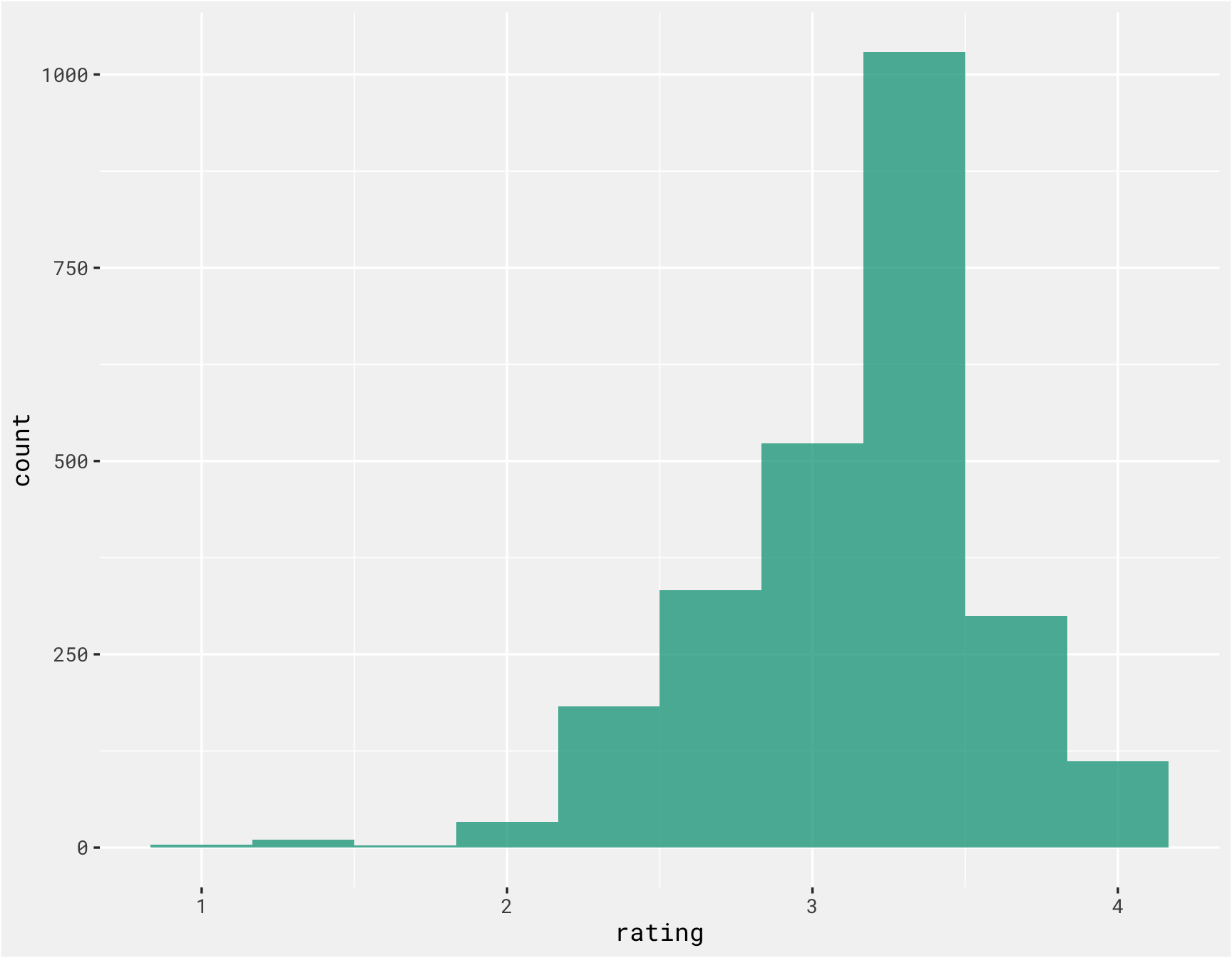
The average rating is around 3.3 or 3.4 out of 5, are ratings are slightly skewed to the left.
chocolate %>%
  ggplot(., aes(x = rating)) +
  geom_histogram(bins = 10, alpha = .75, fill = bg_green) +
  bg_theme()
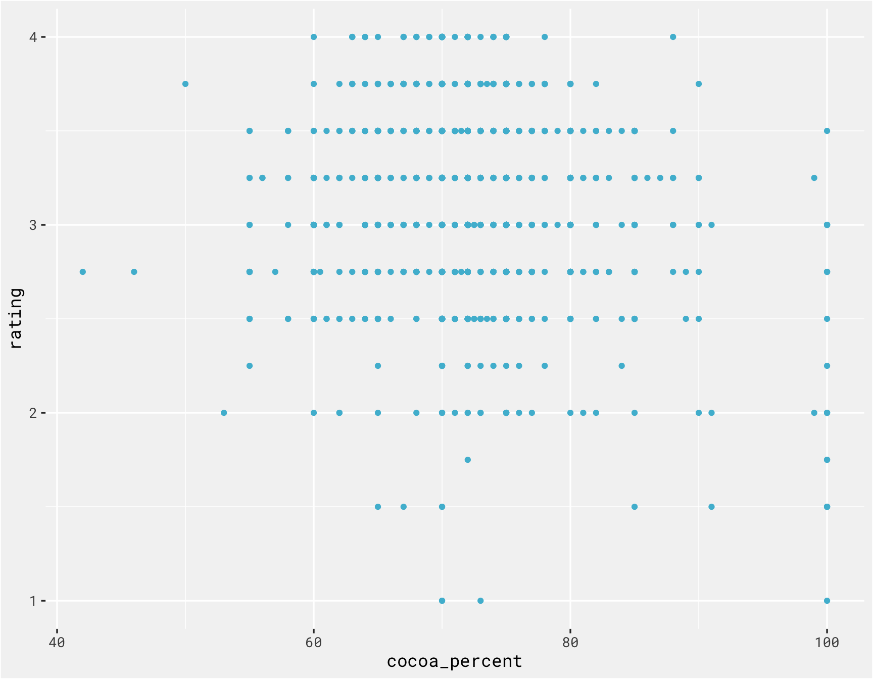
There isn’t much of a relationship between cocoa percent and rating.
chocolate %>%
  mutate(cocoa_percent = as.numeric(str_remove_all(cocoa_percent, "%"))) %>%
  ggplot(., aes(x = cocoa_percent, y = rating)) +
  geom_point(color = bg_blue) +
  bg_theme()
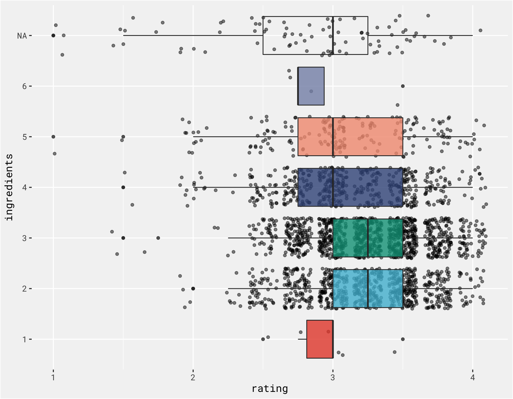
chocolate with 2 and 3 ingredients seem to be rated higher than those with 4 or 5.
chocolate %>%
  mutate(ingredients = substr(ingredients, 1, 1)) %>%
  ggplot(., aes(x = ingredients, y = rating, fill = ingredients)) +
  geom_jitter(alpha = .50, show.legend = FALSE) +
  geom_boxplot(show.legend = FALSE, alpha = .80) +
  bg_theme()  +
  coord_flip() +
  scale_fill_npg()
Model
The most memorable characteristics column will be used along with number of ingredients as predictors of rating. The most memorable characteristics is split and pivoted into indicator variables. A 2nd recipe that includes step_nzv() will also be used to see if removing sparse ingredients improves model performance.
max_characteristics <-
  chocolate %>%
  mutate(num_char = str_count(most_memorable_characteristics, ",") + 1) %>%
  filter(num_char == max(num_char)) %>%
  select(num_char) %>%
  distinct() %>%
  pull(num_char)

choc_characteristics <-
  chocolate %>%
  mutate(ingredients = substr(ingredients, 1, 1)) %>%
  tidyr::separate(most_memorable_characteristics, paste0("characteristic", 1:max_characteristics), sep = ",") %>%
  pivot_longer(cols = starts_with("characteristic"), values_to = "characteristic") %>%
  mutate(characteristic = trimws(characteristic)) %>%
  select(-name) %>%
  filter(!(is.na(characteristic)),
         characteristic != '') %>%
  mutate(characteristic_ind = 1) %>%
  pivot_wider(names_from = characteristic, values_from = characteristic_ind) %>%
  select(rating, ingredient_count = ingredients, `rich cocoa`:ncol(.)) %>%
  filter(!(is.na(ingredient_count)))

choc_characteristics[is.na(choc_characteristics)] <- 0

head(choc_characteristics)
## # A tibble: 6 × 973
##   rating ingredient_count `rich cocoa` fatty bready cocoa vegetal savory
##    <dbl> <chr>                   <dbl> <dbl>  <dbl> <dbl>   <dbl>  <dbl>
## 1   3.25 3                           1     1      1     0       0      0
## 2   3.5  3                           0     0      0     1       1      1
## 3   3.75 3                           0     0      0     1       0      0
## 4   3    3                           0     0      0     0       0      0
## 5   3    3                           0     1      0     0       0      0
## 6   3.25 3                           0     1      0     0       0      0
## # … with 965 more variables: blackberry <dbl>, full body <dbl>, chewy <dbl>,
## #   off <dbl>, rubbery <dbl>, earthy <dbl>, moss <dbl>, nutty <dbl>,
## #   chalky <dbl>, mildly bitter <dbl>, basic cocoa <dbl>, milk brownie <dbl>,
## #   macadamia <dbl>, fruity <dbl>, melon <dbl>, roasty <dbl>,
## #   brief fruit note <dbl>, burnt rubber <dbl>, alkalyzed notes <dbl>,
## #   sticky <dbl>, red fruit <dbl>, sour <dbl>, smokey <dbl>, grass <dbl>,
## #   mild tobacco <dbl>, mild fruit <dbl>, strong smoke <dbl>, green <dbl>, …
Here we prep for modelling by creating splits, resamples and the recipe.
set.seed(163)
splits <-
  choc_characteristics %>%
  initial_split(strata = rating)

train <-
  training(splits)
test <-
  testing(splits)

folds <-
  bootstraps(train, 25, strata = rating)

recipe <-
  recipe(rating ~ ., train)
The same 3 models are used for each workflowset. Here is the ‘regular’ workflowset:
svm_spec <-
  svm_linear(cost = tune(),
              margin = tune()
             ) %>%
  set_mode("regression") %>%
  set_engine("LiblineaR")

workflows <-
  workflow_set(
    preproc = list(recipe = recipe),
    models = list(svm = svm_spec
                  ),
    cross = TRUE)

workflows
## # A workflow set/tibble: 1 × 4
##   wflow_id   info             option    result
##   <chr>      <list>           <list>    <list>
## 1 recipe_svm <tibble [1 × 4]> <opts[0]> <list [0]>
And here is the text-based workflow, adapted from this post.
# text models

set.seed(194)
choco_split <-
  initial_split(chocolate, strata = rating)
choco_train <-
  training(choco_split)
choco_test <-
  testing(choco_split)

choco_folds <-
  bootstraps(choco_train, 25, strata = rating)

choco_rec <-
  recipe(rating ~ most_memorable_characteristics, data = choco_train) %>%
  step_tokenize(most_memorable_characteristics) %>%
  step_tokenfilter(most_memorable_characteristics, max_tokens = 100) %>%
  step_tfidf(most_memorable_characteristics)

text_workflows <-
  workflow_set(
    preproc = list(text_recipe = choco_rec),
    models = list(svm = svm_spec
                  ),
    cross = TRUE)

text_workflows
## # A workflow set/tibble: 1 × 4
##   wflow_id        info             option    result
##   <chr>           <list>           <list>    <list>
## 1 text_recipe_svm <tibble [1 × 4]> <opts[0]> <list [0]>
Here both model types are tuned and compared:
cl <-
  makeCluster(10)

doParallel::registerDoParallel(cl)

grid_ctrl <-
  control_grid(
    save_pred = TRUE,
    allow_par = TRUE,
    parallel_over = "everything",
    verbose = TRUE
  )

results <-
  workflow_map(fn = "tune_grid",
               object = workflows,
               seed = 155,
               verbose = TRUE,
               control = grid_ctrl,
               grid = 10,
               resamples = folds,
               metrics = metric_set(rmse, mae)
  )

stopCluster(cl)
cl <-
  makeCluster(10)

doParallel::registerDoParallel(cl)

grid_ctrl <-
  control_grid(
    save_pred = TRUE,
    allow_par = TRUE,
    parallel_over = "everything",
    verbose = TRUE
  )

text_results <-
  workflow_map(fn = "tune_grid",
               object = text_workflows,
               seed = 155,
               verbose = TRUE,
               control = grid_ctrl,
               grid = 10,
               resamples = choco_folds,
               metrics = metric_set(rmse, mae)
  )
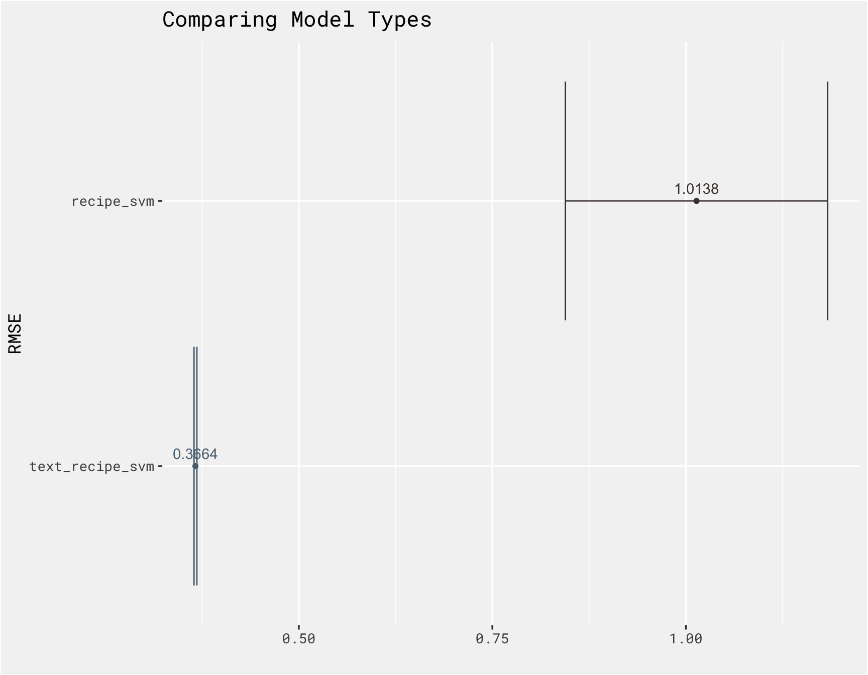
Using a text based approach does perform better in this case! A lot more could probably be done to improve model performance, such as more pre-processing steps, including more predictors, trying various types of models, but the goal of this post was to try out some text based models and see how those models perform to more “traditional” ML models.
results %>%
  rank_results(select_best = T) %>%
  bind_rows(text_results %>% rank_results(select_best = TRUE)) %>%
  filter(.metric == "rmse") %>%
  ggplot(., aes(x = reorder(wflow_id, mean), y = mean, color = wflow_id, label = round(mean, 4))) +
  geom_point(show.legend = FALSE) +
  geom_text(vjust = -0.7, show.legend = FALSE) +
  geom_errorbar(aes(ymin = mean - std_err, ymax = mean + std_err), show.legend = FALSE) +
  bg_theme(base_size = 13) +
  ghibli::scale_color_ghibli_d("PonyoMedium") +
  coord_flip() +
  labs(x = "RMSE", y = '', title = "Comparing Model Types")
- Posted on:
- January 18, 2022
- Length:
- 6 minute read, 1174 words
- Categories:
- tidy tuesday tidymodels data science