Getting started with topic modeling with dog breed traits

Introduction

I first learned about topic modeling after watching this video of Julia Silge creating topic models for Spice Girls lyrics. After checking out this weeks Tidy Tuesday datasets I thought I might try to learn about topic modeling and to develop one using dog breed traits.

Explore the data

breed_traits <-
  readr::read_csv('https://raw.githubusercontent.com/rfordatascience/tidytuesday/master/data/2022/2022-02-01/breed_traits.csv') %>%
  janitor::clean_names() %>%
  mutate(breed = str_squish(breed))

trait_description <-
  readr::read_csv('https://raw.githubusercontent.com/rfordatascience/tidytuesday/master/data/2022/2022-02-01/trait_description.csv') %>%
  janitor::clean_names() %>%
  mutate(trait = str_squish(trait))

breed_rank_all <-
  readr::read_csv('https://raw.githubusercontent.com/rfordatascience/tidytuesday/master/data/2022/2022-02-01/breed_rank.csv') %>%
  janitor::clean_names() %>%
  mutate(breed = str_squish(breed))

breed_traits 

## # A tibble: 195 × 17
##    breed     affectionate_wit… good_with_young_… good_with_other… shedding_level
##    <chr>                 <dbl>             <dbl>            <dbl>          <dbl>
##  1 Retrieve…                 5                 5                5              4
##  2 French B…                 5                 5                4              3
##  3 German S…                 5                 5                3              4
##  4 Retrieve…                 5                 5                5              4
##  5 Bulldogs                  4                 3                3              3
##  6 Poodles                   5                 5                3              1
##  7 Beagles                   3                 5                5              3
##  8 Rottweil…                 5                 3                3              3
##  9 Pointers…                 5                 5                4              3
## 10 Dachshun…                 5                 3                4              2
## # … with 185 more rows, and 12 more variables: coat_grooming_frequency <dbl>,
## #   drooling_level <dbl>, coat_type <chr>, coat_length <chr>,
## #   openness_to_strangers <dbl>, playfulness_level <dbl>,
## #   watchdog_protective_nature <dbl>, adaptability_level <dbl>,
## #   trainability_level <dbl>, energy_level <dbl>, barking_level <dbl>,
## #   mental_stimulation_needs <dbl>

# trait_description <- 
#   trait_description %>% 
#   mutate(trait = stringr::str_to_lower(trait),
#          trait = stringr::str_replace_all(trait, ' ', '_'),
#          trait = stringr::str_replace_all(trait, '/', '_'))

trait_description 

## # A tibble: 16 × 4
##    trait                      trait_1                    trait_5  description   
##    <chr>                      <chr>                      <chr>    <chr>         
##  1 Affectionate With Family   Independent                Lovey-D… How affection…
##  2 Good With Young Children   Not Recommended            Good Wi… A breed's lev…
##  3 Good With Other Dogs       Not Recommended            Good Wi… How generally…
##  4 Shedding Level             No Shedding                Hair Ev… How much fur …
##  5 Coat Grooming Frequency    Monthly                    Daily    How frequentl…
##  6 Drooling Level             Less Likely to Drool       Always … How drool-pro…
##  7 Coat Type                  -                          -        Canine coats …
##  8 Coat Length                -                          -        How long the …
##  9 Openness To Strangers      Reserved                   Everyon… How welcoming…
## 10 Playfulness Level          Only When You Want To Play Non-Stop How enthusias…
## 11 Watchdog/Protective Nature What's Mine Is Yours       Vigilant A breed's ten…
## 12 Adaptability Level         Lives For Routine          Highly … How easily a …
## 13 Trainability Level         Self-Willed                Eager t… How easy it w…
## 14 Energy Level               Couch Potato               High En… The amount of…
## 15 Barking Level              Only To Alert              Very Vo… How often thi…
## 16 Mental Stimulation Needs   Happy to Lounge            Needs a… How much ment…

breed_rank_all

## # A tibble: 195 × 11
##    breed       x2013_rank x2014_rank x2015_rank x2016_rank x2017_rank x2018_rank
##    <chr>            <dbl>      <dbl>      <dbl>      <dbl>      <dbl>      <dbl>
##  1 Retrievers…          1          1          1          1          1          1
##  2 French Bul…         11          9          6          6          4          4
##  3 German She…          2          2          2          2          2          2
##  4 Retrievers…          3          3          3          3          3          3
##  5 Bulldogs             5          4          4          4          5          5
##  6 Poodles              8          7          8          7          7          7
##  7 Beagles              4          5          5          5          6          6
##  8 Rottweilers          9         10          9          8          8          8
##  9 Pointers (…         13         12         11         11         10          9
## 10 Dachshunds          10         11         13         13         13         12
## # … with 185 more rows, and 4 more variables: x2019_rank <dbl>,
## #   x2020_rank <dbl>, links <chr>, image <chr>

Top and bottom 5 breeds based on avg rank 2012-2020

breed_rank_all %>%
  select(-c(links, image)) %>%
  pivot_longer(cols = starts_with("x"), values_to = 'rank') %>%
  group_by(breed) %>%
  summarise(mean_rank = mean(rank, na.rm = T),
            sd = sd(rank, na.rm = T)) %>%
  ungroup() %>%
  arrange(mean_rank) %>%
  mutate(rank = row_number()) %>% 
  filter(rank <=5 | rank >= nrow(.) - 4) %>% 
    add_table(rows = 10)

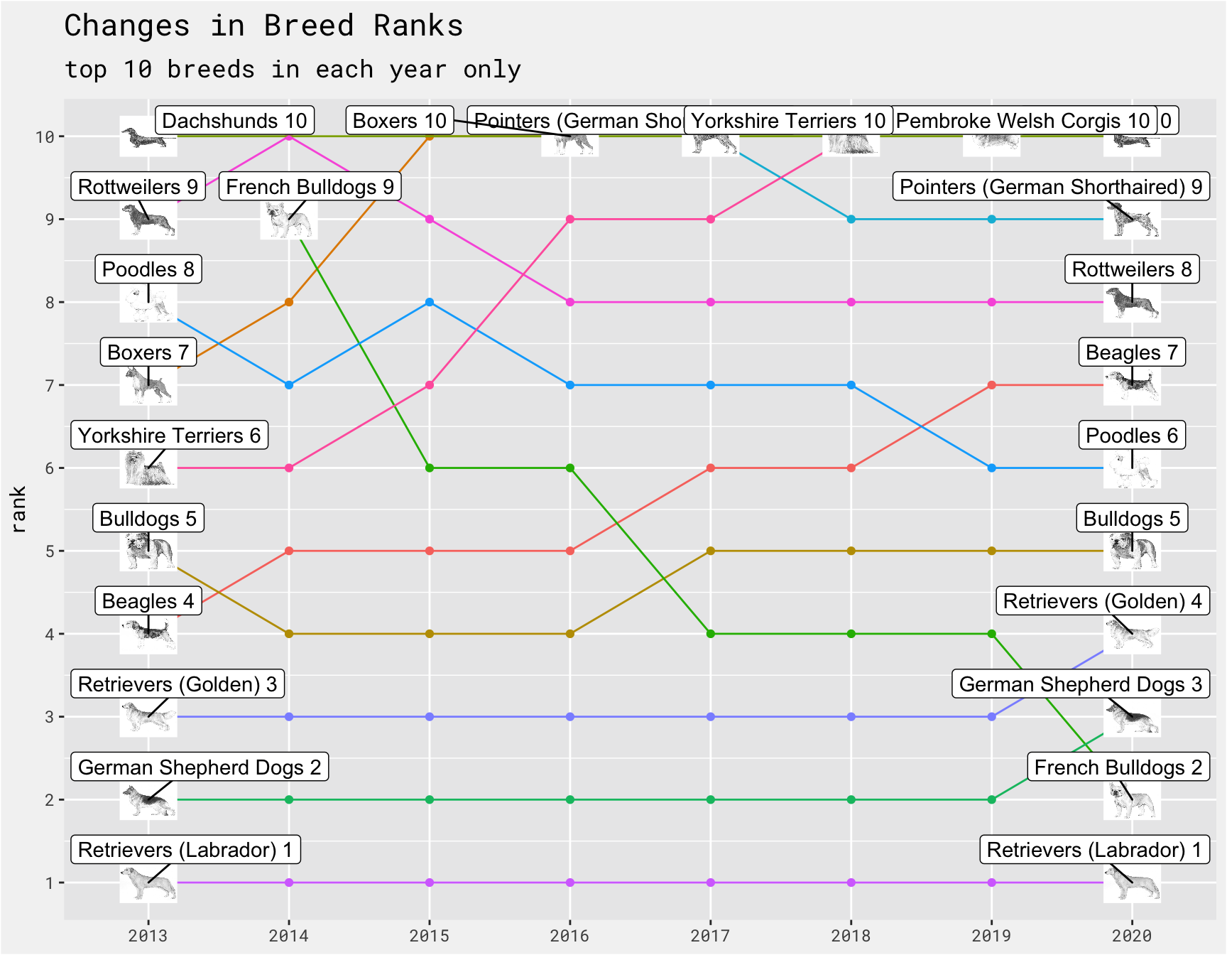
Between 2013 - 2020, Labrador Retrievers were never not #1. French Bulldogs ranking was are most improved from 9 to 2, while Yorkshire Terriers have largest drop from 6 to 10.

breed_rank_all %>%
  # select(-c(links, image)) %>%
  pivot_longer(cols = starts_with("x"), values_to = 'rank') %>%
  mutate(name = str_replace_all(name, "x", ""),
         name = str_replace_all(name, "_rank", ""),
         year = as.numeric(name)
  ) %>%
  select(-name) %>%
  group_by(year) %>%
  mutate(top_15 = ifelse(rank <= 10, 1, 0)) %>% 
  filter(top_15 == 1) %>%
  ungroup() %>%
  group_by(breed) %>%
  mutate(
    label = case_when(
      year == min(year) ~ paste(breed, rank),
      year == max(year) ~ paste(breed, rank),
      TRUE ~ NA_character_),
    image_url = case_when(
      year == min(year) ~ image,
      year == max(year) ~ image,
      TRUE ~ NA_character_)) %>%
  ggplot(aes(x = as.factor(year), y = rank, group = breed, label = label)) + 
  geom_point(show.legend = FALSE, aes(color = breed)) + 
  geom_line(show.legend = FALSE, aes(color = breed)) + 
  geom_image(aes(image = image_url), size=.05) + 
  geom_label_repel(nudge_y = 0.4) + 
  bg_theme() + 
  scale_y_continuous(breaks = seq(1, 10, 1)) + 
  labs(x = NULL, y = "rank", title = "Changes in Breed Ranks", subtitle = "top 10 breeds in each year only") 

mean_rank <- 
  breed_rank_all %>%
  select(-c(links, image)) %>%
  pivot_longer(cols = starts_with("x"), values_to = 'rank') %>%
  group_by(breed) %>%
  summarise(mean_rank = mean(rank, na.rm = T),
            sd = sd(rank)) %>% 
  mutate(breed = trimws(breed),
         breed = as.character(breed)) %>%
  ungroup() %>%
  arrange(mean_rank) %>%
  mutate(rank = row_number()) %>%
  ungroup() %>%
  as_tibble()

traits <- 
  breed_traits %>%
  select(breed, coat_type, coat_length, everything()) %>% 
  ungroup() %>%
  as_tibble() %>%
  pivot_longer(cols = 4:ncol(.), names_to = "trait", values_to = 'trait_score') %>% 
  left_join(., trait_description, by = 'trait') %>%
  ungroup() %>%
  as_tibble() %>% 
  left_join(., mean_rank, by = 'breed')

traits %>% 
  add_table()

Topic Modeling

This dataset gave the opportunity to dive into Text Mining with R to learn more about text analysis and topic modeling.

Topic modeling is a method for unsupervised classification of such documents, similar to clustering on numeric data, which finds natural groups of items even when we’re not sure what we’re looking for.

Next the tidytext’s unnest_tokens() is used to separate the trait descriptions into words, then stop words and some other the common words are removed. This results in a dataframe with 1 word per trait per row. as a first step

trait_list <- 
  c("Affectionate With Family", "Trainability Level", "Barking Level", "Mental Stimulation Needs")

tidy_descripion <-
  trait_description %>%
  filter(trait %in% trait_list) %>%
  unnest_tokens(word, description) %>%
  anti_join(get_stopwords()) %>% 
  filter(!word %in% c("breed", "breeds", "breed's", "dogs"))
  
tidy_descripion %>%
  count(word, sort = TRUE)

## # A tibble: 76 × 2
##    word             n
##    <chr>        <int>
##  1 want             4
##  2 can              3
##  3 bark             2
##  4 dog              2
##  5 everyone         2
##  6 like             2
##  7 others           2
##  8 owner            2
##  9 projects         2
## 10 affectionate     1
## # … with 66 more rows

Next we need to make the data into a DocumentTermMatrix using cast_dtm()

desc_dtm <-
  tidy_descripion %>%
  count(trait, word) %>%
  tidytext::cast_dtm(trait, word, n)

dim(desc_dtm)

## [1]  4 76

This means there are 4 traits (i.e. documents) and 76 different tokens (i.e. terms or words) in our dataset for modeling. Then we use LDA() to create a 4 topic model, one for each of the 4 traits we filtered for above.

# Latent Dirichlet allocation algorithms for topic modelling
traits_lda <- 
  LDA(desc_dtm, k = 4, control = list(seed = 173))

traits_lda

## A LDA_VEM topic model with 4 topics.

we can examine per-topic-per-word probabilities, beta, where the model computes the probability of a given term being generated from a given topic. For example, the term “affectionate” has an almost zero probability of being generated from topics 1, 2, or 3, but it makes up about 5% of topic 4.

# per-topic-per-word probabilities.
trait_topics <- 
  tidy(traits_lda, matrix = "beta")

trait_topics

## # A tibble: 304 × 3
##    topic term              beta
##    <int> <chr>            <dbl>
##  1     1 affectionate 1.67e-146
##  2     2 affectionate 7.24e-146
##  3     3 affectionate 5.37e-146
##  4     4 affectionate 5.88e-  2
##  5     1 aloof        1.67e-146
##  6     2 aloof        7.24e-146
##  7     3 aloof        5.37e-146
##  8     4 aloof        5.88e-  2
##  9     1 best         1.67e-146
## 10     2 best         7.24e-146
## # … with 294 more rows

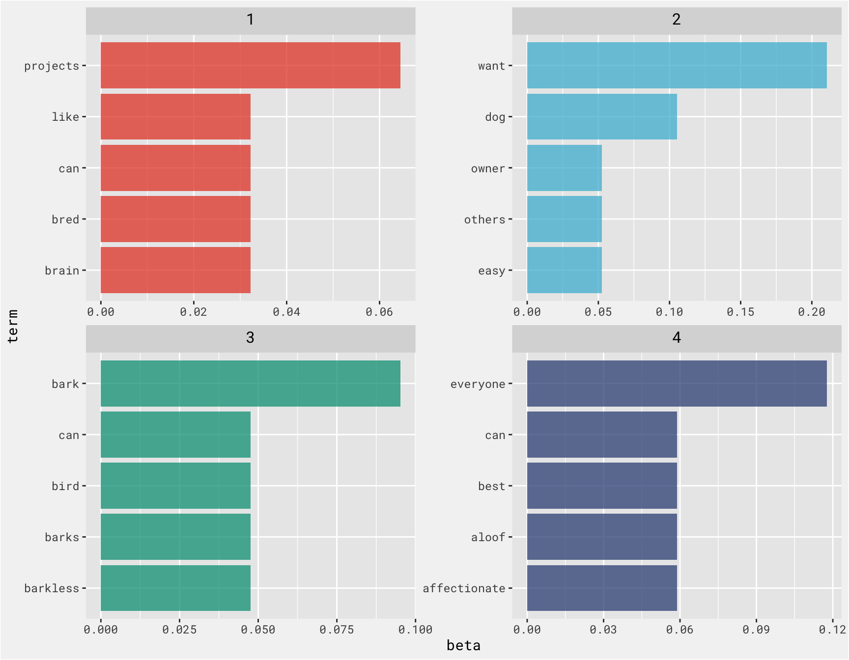
From the plot we can pretty clearly see that topic 1 is probably Mental Stimulation Needs, topic 2 is likely Trainability Level, topic 3 is Barking Level and topic 4 is probably Affectionate With Family

top_terms <- 
  trait_topics %>%
  ungroup() %>%
  group_by(topic) %>%
  slice_max(beta, n = 5, with_ties = FALSE) %>% 
  ungroup() %>%
  arrange(topic, -beta)

top_terms %>%
  mutate(term = reorder_within(term, beta, topic)) %>%
  ggplot(aes(x = beta, y = term, fill = factor(topic))) +
  geom_col(show.legend = FALSE, alpha = .76) +
  facet_wrap(~ topic, scales = "free") +
  scale_y_reordered() + 
  bg_theme() +
  scale_fill_npg()

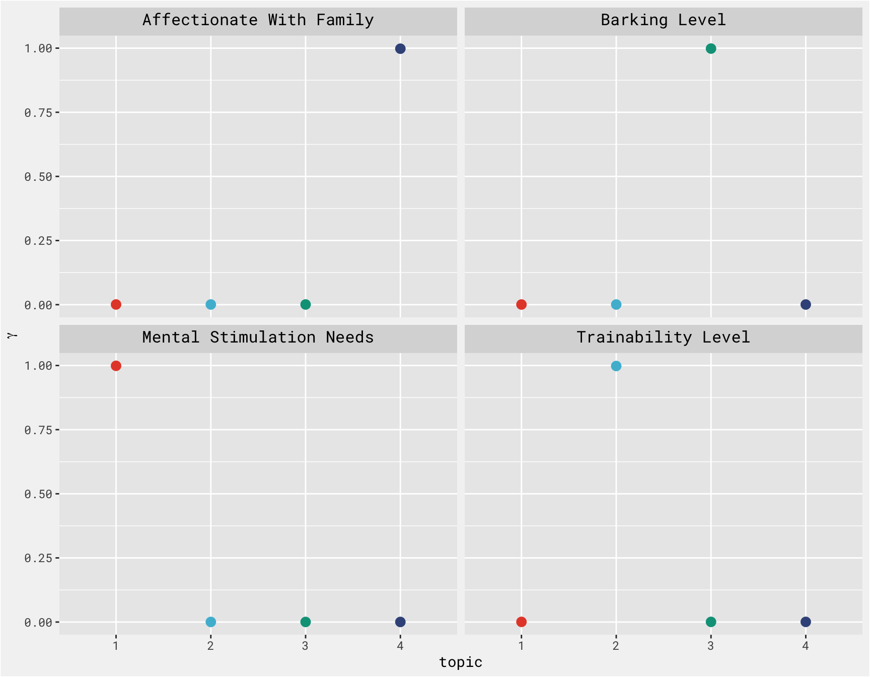
We can then examine per-document-per-topic probabilities, gamma. This lets us take a look at topic probabilities of each trait. This aligns well with the plot above.

traits_gamma <- 
  tidy(traits_lda, matrix = "gamma")

traits_gamma

## # A tibble: 16 × 3
##    document                 topic    gamma
##    <chr>                    <int>    <dbl>
##  1 Affectionate With Family     1 0.000719
##  2 Barking Level                1 0.000582
##  3 Mental Stimulation Needs     1 0.999   
##  4 Trainability Level           1 0.000643
##  5 Affectionate With Family     2 0.000719
##  6 Barking Level                2 0.000582
##  7 Mental Stimulation Needs     2 0.000395
##  8 Trainability Level           2 0.998   
##  9 Affectionate With Family     3 0.000719
## 10 Barking Level                3 0.998   
## 11 Mental Stimulation Needs     3 0.000395
## 12 Trainability Level           3 0.000643
## 13 Affectionate With Family     4 0.998   
## 14 Barking Level                4 0.000582
## 15 Mental Stimulation Needs     4 0.000395
## 16 Trainability Level           4 0.000643

traits_gamma %>%
  ggplot(aes(x = factor(topic), y = gamma, color = factor(topic))) +
  geom_point(size = 3, show.legend = FALSE) +
  facet_wrap(~ document) +
  labs(x = "topic", y = expression(gamma)) + 
  bg_theme() +
  scale_color_npg()